eScience: Chino Hills Earthquake Simulations
Ricardo Taborda, Julio López, Jacobo Bielak
The 2008 Chino Hills earthquake was the largest earthquake in the Los Angeles metropolitan region since the 1994 Northridge earthquake. With a magnitude Mw 5.4, the July 29, 2008 Chino Hills earthquake was recorded by most networks in the area. Its occurrence constitutes an excellent opportunity to study the response of the greater Los Angeles basin and to test the most common assumptions for crustal structure and material properties under ideal conditions of anelastic modeling due to a kinematic point source excitation. We present here a preliminary validation study for a set of simulations of the Chino Hills earthquake using Hercules—the parallel octree-based finite element simulator developed by the Quake Group at Carnegie Mellon University. In the past, we have reported on the simulation capabilities of Hercules for more complex—yet hypothetical—earthquake scenarios such as TeraShake and ShakeOut. For the latter, we have also conducted a comprehensive verification of results obtained from different simulation methodologies such as finite elements and finite differences. The verification was performed in collaboration with other simulation groups from the Southern California Earthquake Center (SCEC). With this new simulation we attempt to come full circle in the verification and validation paradigm as understood by the modeling and simulation community. The results presented here correspond to a set of four different simulations, the most challenging one with a maximum frequency of 2 Hz and a minimum shear wave velocity of 200 m/s. These particular values of these two critical parameters help us explore the influence of higher frequencies and lower velocity profiles on ground motion. The extension to these parameters is becoming possible in our simulations thanks to the latest computational improvements we are implementing into Hercules. While our focus is on the physical interpretation of the results of our simulations and their comparison with observations, we also report on the computing resources employed. Our preliminary results suggest that extending the maximum frequency beyond the "de facto" assumed barrier of 1 Hz for deterministic simulations is an effort worth pursuing.
The Earthquake and Simulation Model
The Chino Hills earthquake (Mw 5.4) of July 29, 2008 was the strongest earthquake in the greater Los Angeles metropolitan area since Northridge in 1994. Because it can still be considered a relatively minor earthquake, its occurrence constitutes an excellent opportunity to test the simulation capabilities in continuous development within SCEC.
A preliminary report from USGS and CalTech scientists [1] indicated that the source was at about 15 km depth between the Whittier and Chino faults west of Los Angeles. The epicenter is shown Figure 1. This figure also includes the major cities in the region and mapped quaternary faults, as well as the the surface projection of the model domain used for the simulation.
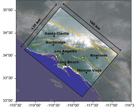 |
| Figure 1. Region and simulation domain including the epicenter and major cities. |
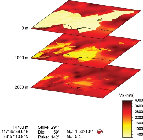
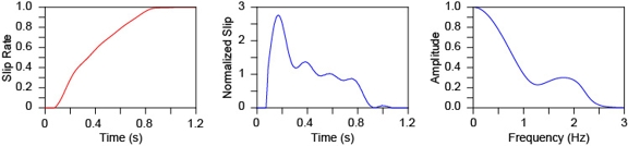
The focal mechanism and properties of the earthquake source are described in Figure 2. We modeled it as a point source with the normalized slip function and slip rate shown in Figure 3. The final dislocation was set to match the seismic moment Mo = 1.53×10¹⁷ Nm. Figure 2 also shows a schematic representation of the material model used for the simulation: an etree [2] representation of SCEC's Comunity Velocity Model (CVM-S, version 4.0.)
|
| Figure 2. Material model description and location and characteristics of the source. |
|
| Figure 3. Normalized slip function and corresponding slip rate and slip rate magnitude spectrum. |
The simulation was done using Hercules [3], an octree-based finite element parallel code developed by the Quake Group at Carnegie Mellon University for solving forward seismic wave propagation problems due to kinematic faulting. Hercules capabilities have been thoroughly tested and verified [4]. The simulation parameters and model characteristics are listed in Table 1. We want to highlight that the unstructured mesh built to represent the system is valid for frequencies up to 2 Hz and shear wave velocities (Vs) down to 200 m/s.
Table 1. Simulation parameters and model characteristics.
| Maximum frequency | 2 Hz |
| Minimum Vs | 200 m/s |
| Domain size | 180 × 135 × 62 km3 |
| Simulation Δt | 0.001 s |
| Simulation time | 100 s |
| Total time steps | 100,000 |
| Points per wavelength | 8 ≤ p < 14 |
| Spatial discretization | Second Order |
| Time discretization | Second Order |
| Meshing Octree | FEM |
| Number of nodes | 708,266,881 |
| Number of Elements | 630,618,239 |
High-Performance Computing
Hercules [3] is a highly computationally efficient code for end-to-end earthquake ground motion simulations. We take advantage of a database library developed in-house [2] to store the material model in an etree format to build large meshes in minimum time. Our octree-based finite element approach is wave-length adaptive thus the number of elements is also optimized according to material properties. We have also tuned up the core solver in the code to run at a high speed and expect to continue improving other aspects of it. Table 2 shows the performance achieved for simulating the Chino Hills earthquake for the physical characteristics listed in Table 1.
Table 2. Computational performance achieved
running in Kraken (Cray XT5) at NICS.
| Number of cores | 4,096 | |
| Total running time | 63,858 s | 17:44:18 |
| – Meshing time | 642 s | 10:42 |
| – Solving time | 63,216 s | 17:33:36 |
| – Core solver time | 35,684 s | 9:54:44 |
| – Balancing time | 2,731 s | 45:31 |
| – IO time | 1,877 s | 31:17 |
| Total service units (SU) | 72,656 |
Simulation Results and Validation
Figure 4 shows the progress of the seismic waves as they are emanated from the source rupture and travel throughout the region. As has been observed in other similar simulations, waves are clearly amplified by the basin and guided by the different features of the geologic model. However, only now that we have the capability of extending the maximum frequency to higher and more realistic values and lower the shear-wave velocity to one characteristic of soft deposits, can we observe the kind of spatial variability reported from past earthquakes.
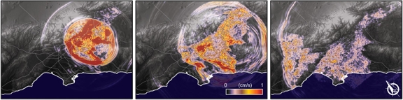 |
| Figure 4. Simulation snapshots of surface horizontal magnitude velocity for time t = 9.8 s (left), 17.3 s (center), and 30 s (right). The maximum value of horizontal magnitude velocity obtained in the simulation was 35.76 cm/s. Here the color limit is set at a lower value for visual convenience. |
This is key if we want to make use of a physics-based approach to earthquake hazard analysis. Nevertheless, validation is required. Towards this end we selected 65 stations from the CI strong motion network (using the STP service of the SCEDC) for direct comparisons with the simulation. These recording locations are shown in Figure 5.
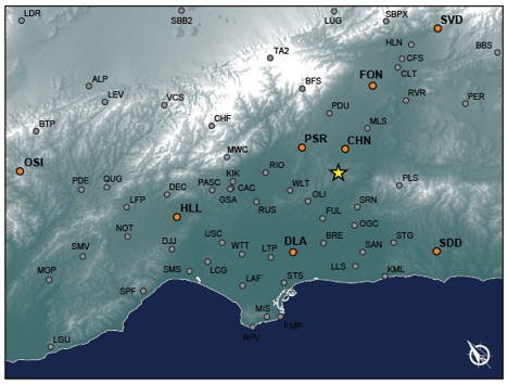 |
| Figure 5. All 65 stations selected from the CI network for comparisons between data and synthetics. Those used for Figure 6 are highlighted. |
A direct comparison between synthetics and data for a subset of the stations is shown in Figure 6 for the ground velocity in the two horizontal components. Also included in the figure is a comparison of the spectra of each couple of traces.
|
| Figure 6. Comparison between synthetics (red) and data (blue) for the surface velocity (left) and the corresponding Fourier transform (right) at eight stations for the EW (090) and NS (000) components of motion. andfor particle velocity (in cm/s) at eight locations for each component of motion. Peak velocity values are shown to the right of each trace set. The stations are divided in 4 different groups depending on the similarity of the simulation results with respect to strong motion recordings. |
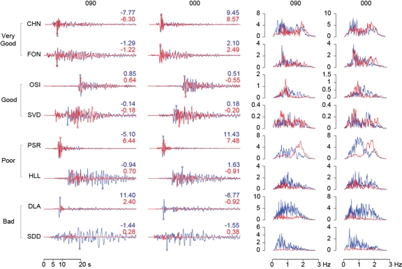
We divided the results into four categories ranging from very good to bad. Based on the features of the signals and spectra of those stations we labeled as good or very good, we believe that our simulation makes a good case for continuing to pursue the goal of extending the maximum frequency for deterministic simulations beyond the "de facto" assumed barrier of 1 Hz. Doing so will help us better characterize the expected ground response in the region and complement the information gathered from strong motion networks.
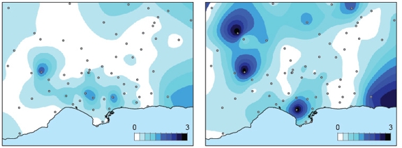
Figure 7 compares the ShakeMap data distributed by the USGS and the equivalent result obtained from the simulation. The ShakeMap is produced by interpolating the data recorded at all available stations scattered throughout the region. Thus, it does not capture the spatial variability that is visible northeast of the epicenter in the simulation results. At the same time, south of the epicenter, the simulation data contains sharp edges resulting from the material model (see Figure 2), which raises legitimate questions. The same effect is shown in the seismograms at the bottom of Figure 6.
|
| Figure 7. Comparison of results for the peak horizontal ground velocities between the simulation (left) and the USGS ShakeMap (right) [1]. Simulation results are limited to the modeling parameters whereas the ShakeMap results correspond to an interpolation of actual recorded data at all that stations in the region that recorded the event. |
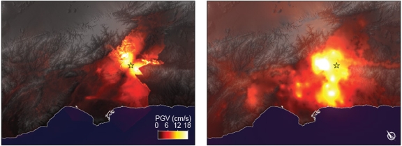
However, it is difficult to settle for a cause to the discrepancies. Differences in the spectra and the signals indicate a better source representation is needed. Synthetics dying out faster than records may suggest that a better attenuation model would help as well. And abrupt changes as those observed in Figure 7 (left) reveal that the material model is a key factor.
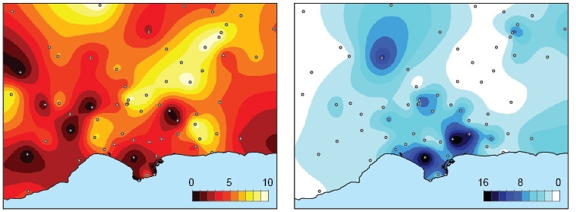
To elucidate this matter, some metrics of the comparisons can help. Figure 8 (left) shows contours drawn using the results from running a goodness-of-fit (GOF) criteria for peak ground velocities [5]. This and other similar criteria are very useful to combinedly grade synthetics. However, this one in particular gives no information about when the peak velocities occur. To overcome this we complement it by plotting the corresponding contours for the difference between the times at which peak values occur. Figure 8 shows that a synthetic may have a very similar peak value (which would result in a good GOF score) but occur at a very different time. Conversely, a bad GOF score would hide positive aspects like the peaks ocurring at the same time—regardless of their difference in magnitude.
|
| Figure 8. Left: Goodness-of-fit scores for peak ground velocities (C6 on [5]). A score of 10 represents a perfect match. Right: Absolute difference (in seconds) between the times at which peak velocities are observed. A difference of zero means that peak values in both the synthetics and the data occurred at the same time. |
For this reason we believe that other measures should also be considered. Figure 9 shows a measure of the error in the time of the first arrival of P- and S-waves in the synthetics with respect to the stations data. We believe this kind of metrics add more to the comparison because they give insight on how to improve the material and source models.
|
| Figure 9. Contours of the absolute difference (in seconds) for the times at which the first P-waves (left) and S-waves arrive at the selected stations in the simulation with respect to the recorded data. A difference of zero means that first wave arrivals in the simulation occurred at the same time as in the data. |
Conclusions
In the last five years SCEC's Comunity Modeling Environment group has achieved remarkable landmarks in regional earthquake simulations from TeraShake to ShakeOut. Collaborating within CME, our group has been at the forefront of pushing the boundaries of physics and computational challenges in earthquake ground motion simulations. The present simulation is yet another step in contributing through SCEC to move us forward toward a physics-based approach to seismic hazard analysis. We believe that as we continue to improve all other aspects of simulation (source description and material models) the computational capability of codes like Hercules will rise to the challenge posed by engineering needs, as well as help us better understand the seismic response of earthquake prone regions.
REFERENCES
[1] Hauksson E, Felzer K, Given D, Giveon M, Housh S, Hutton K, Kanamori H, Sevilgen V, Wei S and Young A (2008). Preliminary report on the 29 July 2008 Mw 5.4 Chino Hills, eastern Los Angeles basin, california, earthquake sequence. Seismological Research Letters, 79(6) 855–866.
[2] Tu T, O'Hallaron D and Lopez J (2003). The Etree Library: A system for manipulating large octrees on disk. Technical Report CMU-CS-03-174, School of Computer Science, Carnegie Mellon University.
[3] Tu T, Yu H, Ramirez-Guzman L, Bielak J, Ghattas O, Ma KL and O'Hallaron D (2006). From Mesh Generation to Scientific Visualization: An End-to-End Approach to Parallel Supercomputing. Proceedings of SC2006, Tampa, Fl, November, 2006.
[4] Bielak J, Graves R, Olsen K, Taborda R, Ramírez-Guzmán L, Day SM, Ely GP, Roten D, Jordan TH, Maechling PJ, Urbanic J and Juve G (2009). The ShakeOut earthquake scenario: Verification of three simulation sets. Geophysical Journal International, Submitted for publication March 17, 2009.
[5] Anderson J (2004). Quantitative measuro of the goodness-of-fit of synthetic seismograms. Proceedings of the XIII World Conference on Earthquake Engineering, Vancouver, Canada. Paper No. 243.
People
FACULTY
Jacobo Bielak (CEE CMU)
Julio López
GRAD STUDENTS
Haydar Karaoglu (Ph.D student, CEE CMU)
COLLABORATORS
Ricardo Taborda (post-doc CEE CMU)
Leonardo Ramírez-Guzmán (Ph.D. USGS)
Acknowledgements
This research is supported in part by the Gordon and Betty Moore Foundation, in the eScience project. The computations were supported by an allocation of advanced computing resources provided by the NSF and performed on Kraken at the National Institute for Computational Sciences.
We thank the members and companies of the PDL Consortium: Amazon, Bloomberg LP, Datadog, Google, Honda, Intel Corporation, Jane Street, LayerZero Research, Meta, Microsoft Research, Oracle Corporation, Oracle Cloud Infrastructure, Pure Storage, Salesforce, Samsung Semiconductor Inc., and Western Digital for their interest, insights, feedback, and support.